Magical Power of Quantum Mechanics

Standing on the Shoulders of Giants Hammond’s Postulate

QM Magic Class | Chapter 8

n previous chapters, we have introduced the application of HOMO/LUMO analysis of heterocycle substrates to rationalize reaction outcome, make quick prediction, and facilitate synthetic planning.

In our laboratory practice, we found that there are occasions in which further calculations for reaction energy profile and transition state are necessary to provide quantitative estimate for selectivity in reaction, and to gain deeper insights on reaction mechanisms.

Today, we would like to review three key theories which laid the foundation of reaction energy calculations.

1889 • Arrhenius Equation

How can a chemical reaction take place? What controls the reaction rate and determines the product selectivity? In 1889, Svante Arrhenius first proposed an empirical formula that summarizes the relationship between reaction rate and temperature, which is now well-recognized as Arrhenius Equation (Figure 1).

Figure 1. Empirical Arrhenius Equation

It states that for reactants to transform into products, they must first acquire a minimum amount of energy, activation energy Ea. When a reaction has a rate constant that obeys Arrhenius Equation, a plot of lnk versus T⁻¹ gives a straight line (Arrhenius plot). By measuring a set of reaction rates under different temperature, one can determine the activation energy Ea and pre-exponential factor A from the slope and the intercept, respectively.

The Arrhenius Law was derived from experimental data with absolutely a wide range of successful applications. However, macroscopic observations cannot always explain microscopic events. The fact that it lacks mechanistic considerations on individual molecular behaviors urged further interpretations and developments therefrom.

1935 • Transition State Theory

n 1935, benefit from significant development of statistical thermodynamics, Henry Eyring et al. proposed the Transition State Theory, along with the Eyring Equation (Figure 2), provided a more sophisticated formula, and addressed the physical interpretations of two parameters in Arrhenius Law:

Figure 2. Arrhenius Equation versus Eyring Equation

Activation Energy: Eyring et al. argued that the reaction does not occur by simple collisions, instead, it requires the formation of an activated transition state complex from reactant molecules. The energy required for reactant molecules to form the transition state complexes is the activation energy. The Gibbs Free Energy of Activation, ΔG^‡, was meantime introduced to account for both enthalpy and entropy changes. For multi-step complex reactions, each transition state should have a corresponding ΔG^‡.

Pre-exponential Factor: it is a function of temperature, representing the frequency with which the activated transition state complexes are converted into products.

In the progress of forming a transition state complex, the potential energy of the entire system changes correspondingly. A chemical reaction could then be described as a moving point over the potential energy surface with coordinates in atomic momenta and distances. Transition State Theory states that the saddle point, i.e, the minimax point, on a potential energy surface, is the transition state of the reaction. For example, as shown in Figure 3, a stable reactant X sits in a local minimum of the potential energy surface. By following different energy paths, distinct transition state complexes are formed at saddle points, leading to products A or B.

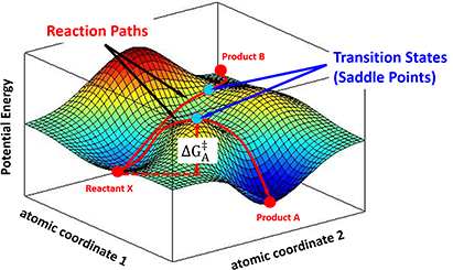
Figure 3. Different reaction paths over a potential energy surface

 In principle, by constructing a potential energy surface from microscopic quantities, one can calculate the absolute reaction rate constants for the reaction; although in practice, it is never easy to obtain the precise knowledge of a potential energy surface. Nevertheless, the concept of “activated transition state complex” has been well accepted since then.

1955 • Hammond's Postulate

In 1955, George Hammond proposed a hypothesis which is of profound significance:

“If two states, as, for example, a transition state and an unstable intermediate, occur consecutively during a reaction process and have nearly the same energy content, their interconversion will involve only a small reorganization of the molecular structures.”

In a one-step reaction, it could be further interpreted as “the structure of a transition state resembles the side of the reaction that is higher in energy.” For a highly exothermic reaction (Figure 4, Left), the transition state is close to the reactant in terms of energy, therefore the structure of the transition state is similar to the reactant. Whereas in an endothermic reaction (Figure 4, Right), the transition state structure resembles the product as now they are closer in energy.

Figure 4. Hammond’s Postulate interpretation in one-step reactions

Transition states are extremely short-lived, roughly at picosecond level, rendering great experimental challenges to capture or to observe. Thus, the postulate provides a geometric model for the transition state complex, enabling chemists to predict its properties by characterizing the known molecules, and modeling the reaction progress.

Figure 5. Calculate product ratio from activation energy difference

In kinetic-controlled reactions, products concentration is proportional to reaction rates, which can be calculated from activation energy difference according to Arrhenius Law, as shown in Figure 5, which is the core equation we will use, for product selectivity predictions in following articles. Whereas in thermodynamic-controlled reactions, the product ratio could be directly obtained from the potential energy differences (between the products and the reactants) ratio.

Standing on the Shoulders of Giants

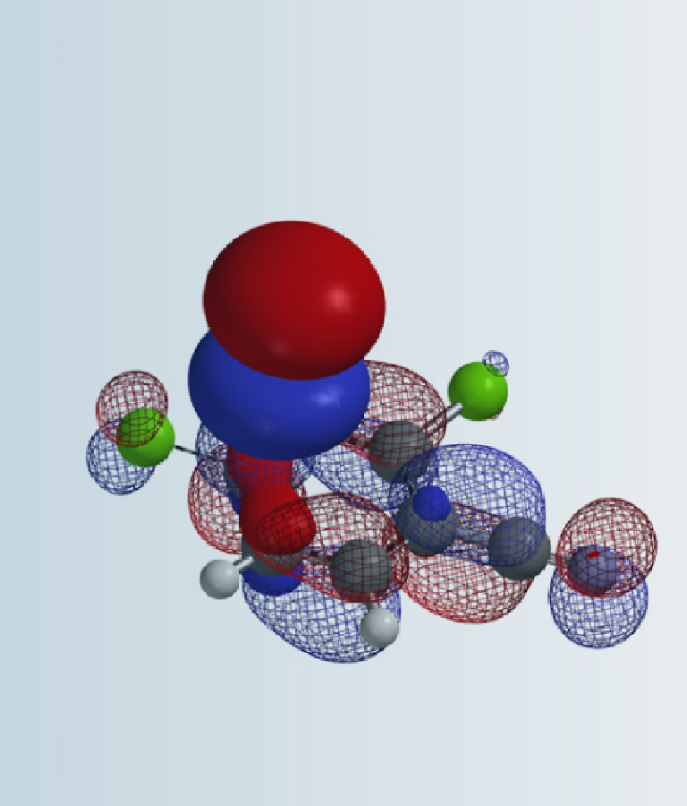
Transition states often involve bond breaking and formation. While Quantum Mechanics is down to the fundamentals of electron behaviors, not limited by arbitrary bond definitions, making it a perfect tool for transition state modeling.

We appreciate those efforts and dedications contributed by generations of scientists into the development of theories for understanding chemical reactions. We also realize that we are all standing on the shoulders of giants.

Combining Frontier Molecular Orbital Theory and Hammond’s Postulate, with increasingly faster computing tools, we now could model the transition state complexes at molecular level. These retrospective analyses provide us with deeper mechanistic insight of the reactions and enable us to analyze chemistry prospectively in a more fundamental manner.

This article is written and edited by Guqin Shi, Wang Shouliang, Wang Qiuyue, and John S. Wai.

References:

[1] Fu Xiancai et al (2006). Physical Chemistry. Beijing, P.R. China: Higher Education Press.

[2] Y. Wang (2014). First principles process planning for computer-aided nanomanufacturing In J. G. Michopoulos, C. J. J. Paredis, D. W. Rose, J. M. Vance (Ed.), Advances in Computers and Information in Engineering Research, Volume 1. New York, NY, USA: ASME Press.

[3] H. Eyring. J. Chem. Phys. 1935, 3, 107-115

[4] G. S. Hammond. J. Am. Chem. Soc. 1955, 77, 334-338

[5] W. J. Hehre, A. J. Shusterman, W. W. Huang (1998). A Laboratory Book of Computational Organic Chemistry. Irvine, CA, USA: Wavefunction, Inc.